Understanding Fourier Feature Mapping Through Simple Image Regression Examples
Introduction
In the realm of neural networks, particularly Multilayer Perceptrons (MLPs), capturing high-frequency signals in data remains a challenging task. This article delves into Fourier feature mapping, a technique used to enable neural networks, especially MLPs (multilayer perceptions), to better capture high-frequency signals in data, particularly in low-dimensional domains such as image and graphics processing.
Imagine a neural network trained to map 2D pixel coordinates (x, y) to RGB color values in an image. This process involves translating low-dimensional input (2D coordinates) into high-frequency output (color variations).
The Challenge with Standard MLPs
A typical MLP, working directly with these coordinates, often falters in capturing image details like sharp edges or fine textures. This ‘spectral bias’ makes MLPs inherently better at learning low-frequency functions.
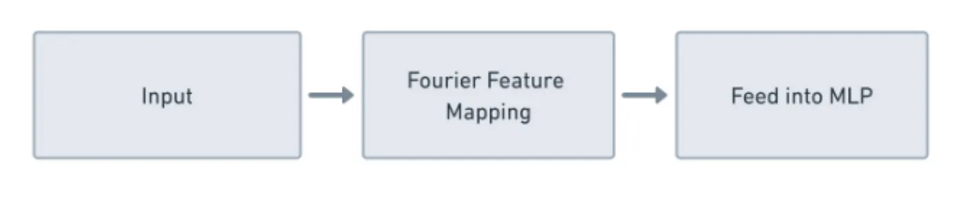
Fourier Feature Mapping: The Concept
To address this limitation, Fourier feature mapping is applied to the input coordinates before they are fed into the MLP. This mapping involves transforming each input coordinate pair (x, y) using a series of sinusoidal functions (sine and cosine) with varying frequencies.
Illustrative Example: A 2x3 Image
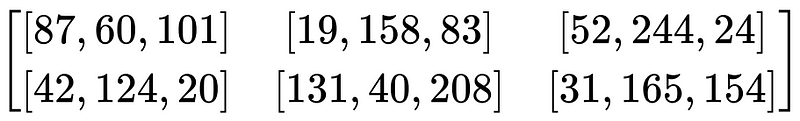
Consider a simple 2x3 image, where each pixel has an RGB value.
The image array looks like this:
The coordinates for these pixels can be represented as (row, column) pairs, starting from (0,0) for the top-left pixel.
Step-by-Step Process
Step 1: Assign Coordinates
We assign coordinates to each pixel:
- Row 0: (0,0), (0,1), (0,2)
- Row 1: (1,0), (1,1), (1,2)
Step 2: Fourier Feature Mapping
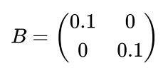
Let’s define a simple 2x2 Fourier mapping matrix ( B ). For simplicity, we will use:
Now, apply the Fourier feature mapping to each coordinate.
Step 3: Apply Mapping to Each Coordinate
For each pixel coordinate, ( v = (x, y) ), compute ( Bv ) and then apply the sinusoidal functions. Let’s do this for the first pixel at (0,0):
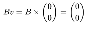
So,

You would repeat this process for each pixel coordinate, computing a transformed vector (gamma(v) ) for each. This mapping enriches the coordinates, preparing them for the MLP.
Step 4: MLP Training
For MLP training, each pixel’s transformed coordinates ( gamma(v) ) are associated with its RGB value. For instance, for pixel (0,0) with RGB [87, 60, 101], the training pair would be:
- Input: [0, 1, 0, 1]
- Output: [87, 60, 101]
You’ll create such pairs for all six pixels.
Step 5: Training the MLP
The MLP is trained on these pairs. Through training, it learns the relationship between the Fourier-transformed coordinates and the RGB values. This step-by-step process shows how Fourier feature mapping transforms simple coordinates into a format that helps an MLP learn complex relationships within image data. Each step is crucial in ensuring the MLP captures the high-frequency details present in the image.
Results
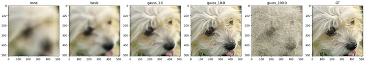
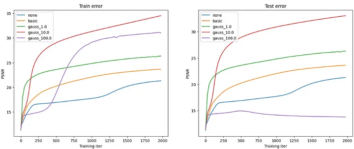
An image of a dog was used for training with different mappings( gamma(v)) :
Try it out your self: open in colab
Conclusion
So, in essence, Fourier feature mapping acts as a pre-processing step that significantly enriches the input data, making it more amenable for neural networks to learn complex, high-frequency patterns, especially in fields like computer vision and graphics.
Reference
This discussion draws its inspiration from the work presented in the paper ‘Fourier Features Let Networks Learn High Frequency Functions in Low Dimensional Domains’. Full credit goes to the original authors for their research in this area. This article aims to facilitate understanding of the concepts introduced in their paper. For comprehensive details and in-depth insights, readers are encouraged to refer directly to the original paper.